Emre: What is this thing called Bayesian inference?

Kaan: I can explain it through an example.

Bayesian inference is a probabilistic approach. To give some information about what it is, we can consider the linear-regression problem. Namely, simple linear regression is a method that allows analysing the linear relationship between two variables in order to predict the value of a dependent variable based on the value of an independent variable. In real life and in machine-learning problems this relationship is generally a statistical one. However, before getting to the essence of how we think about statistical relationships, we need to look at the situation in which the relationship between the two variables is deterministic. In the deterministic case there is always an equation that precisely defines the relationship between the two variables.

Problem

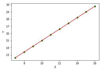
For example, suppose we need to take a taxi from home to the airport. Let’s say the taxi will take 7 TL as a flag-drop fee and will charge 0.8 TL per kilometre (km) during the trip. To find the total cost of our journey, we can set up a linear equation. If $X$ represents the distance travelled in kilometres and $Y$ represents the total cost of the ride, the linear equation is

\[Y = 7 + 0.8 * X\]

When we know the equation deterministically, we can calculate the cost of all trips taken with the same taxi service exactly. If we know the equation, when the data are visualised they look like this:

Classical Linear Regression

Now let’s see what the statistical approach looks like. Suppose we are again in the taxi, but this time we do not know the flag-drop fee or the cost per km. Nevertheless, in order to calculate the cost of future trips we want to estimate the linear equation that the taximeter uses. Suppose we ignore the digits after the decimal point that appear on the taximeter display and write down only the integer part of the cost per km. At this point our task is to fit a line to the points we have noted in order to find the parameters of the following equation:

\[Y = \theta_{0} + \theta_{1} * X\]

The figure below shows the line that fits the points we noted when this problem is solved statistically.

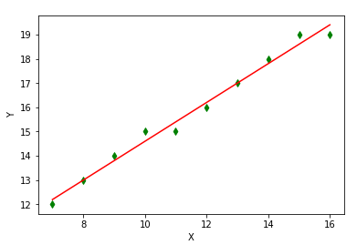
The parameter values we estimate will be

\[\hat{Y} = 6.6 + 0.8 * X\]

so that $\theta_{0} = 6.6$ and $\theta_{1} = 0.8$.

Wait a second, how did we obtain this estimate?

Actually the least-squares method in the context of linear regression has been extensively covered in the literature; therefore I will not go into the details of the algorithm here. However, to build up our story I need to remind some fundamentals.

Since we assume we do not know the deterministic equation, we will use a statistical approach to predict the $Y$ values. The first thing we need to do is to use all the information we have about what the linear relationship between $X$ and $Y$ will be. By looking at how the data are distributed on a two-dimensional plane, we can see that they can be expressed more accurately by a line equation than by a curve equation. In that case our model will be

\[\hat{y_i} = \theta_0 + \theta_1 x_i + \epsilon_i\]

where $\hat{y_i}$ represents the prediction for the $i$-th observation and $\epsilon_i$ represents the error (or “residual”) for the $i$-th observation.

If we express the prediction $\theta_0 + \theta_1 x_i$ as $\theta^T x_i$, the error—computed as the difference between the true value $y_i$ and the prediction $\hat{y_i} = \theta^T x_i$—becomes

\[\epsilon_i = y_i - \hat{y_i} = y_i - \theta^T x_i.\]

The error term is a measure of the part of the linear relationship that our model cannot explain. In linear regression our goal is to find the best-fitting equation that minimises cost functions associated with these errors (Mean Absolute Error, Mean Squared Error, Root Mean Squared Error, etc.). In this context, if we define the Residual Sum of Squares (RSS) as

\[g(\theta) = \sum_{i=1}^{n} (\epsilon_i)^2 = \sum_{i=1}^{n} (y_i - \hat{y_i})^2 = \sum_{i=1}^{n} (y_i - \theta^T x_i)^2,\]

the least-squares fitting method, which has at least one solution for our problem, tries to minimise the RSS:

\[J(\theta_1, \theta_2) = \underset{\theta_1, \theta_2}{\arg\min} \sum_{i=1}^{n} (y_i - \hat{y_i})^2 = \sum_{i=1}^{n} (y_i - \theta^T x_i)^2.\]

Emre: What is this equation trying to do?

Kaan: It sums the squares of the differences and minimises them over the $\theta$ parameters.

Emre: Why do we take squares?

Kaan: Because we do not care about the direction of the error and we don’t want the errors to cancel each other when summed. Nevertheless, our hope and assumption is that the average (expected value) of these errors is zero. This is important for the assumptions we make about our model. Anyway, I will come back to this assumption and explain why it matters later.

Emre: What does it mean to minimise the RSS over the $\theta$ parameters?

Kaan: We differentiate the cost function and set the derivative equal to zero, and solve the equation for the parameter vector $\theta$. The parameter values that make the derivative zero actually give us the point where the derivative of the cost function is zero—in other words, the minimum of the cost function. This is the closed-form solution to our problem. Alternatively we could have used the “Gradient Descent” algorithm. In gradient descent, the minimum of a convex cost function is found by following the gradient iteratively.

Emre: One moment, what exactly is a “gradient”?

Kaan: The gradient is the vector that contains the partial derivatives with respect to each unknown.

Emre: What do we do with these derivatives?

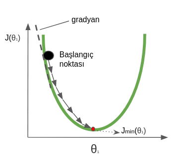
Kaan: The gradient tells us in which direction we should move to reach the minimum. For example, the algorithm starts at a random point on the cost function; the derivative tells us whether to move right or left on the curve. If the derivative is negative we move right and increase $\theta$; if it is positive we move left and decrease $\theta$. We continue this process until we reach the minimum. When we reach the minimum the derivative takes the value zero. Instead of waiting to reach zero, we can also end the algorithm early by putting a threshold close to zero.

The figure below shows how the “Gradient Descent” method reaches the minimum point on a convex function for a single parameter.

On the other hand, in our example there was only one predictor variable $X_1$ and two unknown parameters ($\theta_0$, $\theta_1$). In real-world problems, however, the number of predictor variables can be very large. If we were trying to predict the price of a used car, for instance, there would be many variables such as the brand, model, mileage, safety equipment, etc., which would turn the problem from a simple regression problem into a multiple regression problem. In that case our model would be

\[\hat{y_i} = \theta_0 + \theta_1 x_1 + \theta_2 x_2 + \dots + \theta_p x_p.\]

This is no longer a simple linear-regression problem but a “multiple regression” problem. Working in high dimensions makes taking derivatives quite difficult, so we usually work continuously with gradients. As in the previous example, a method that stops the iteration when the gradient falls below a threshold is used to search for the optimal point.

In general, in multiple regression the gradient is expressed as

\[\nabla J(\theta_1, \dots, \theta_p) = \begin{bmatrix} \frac{\partial J}{\partial \theta_0} \\ \frac{\partial J}{\partial \theta_0} \\ \vdots \\ \frac{\partial J}{\partial \theta_p} \end{bmatrix}.\]

Emre: What does all of this have to do with “Bayesian Inference”?

Statistical Approach

Kaan: Yes, now let’s come to solving the linear-regression problem with a Bayesian approach. To be able to solve the problem with a Bayesian approach we first need to think of the problem as a statistical problem.

Emre: What do you mean?

Kaan: Instead of a “curve fitting” that minimises the cost function, this time we need a “curve fitting” that maximises the likelihood of the observations we have. In general, using our assumptions about how the data come into being, we can calculate the likelihood of the data as

\[L \text{ (likelihood)} = p(y | x) = p(y_1 | x_1, \theta) * p(y_2 | x_2, \theta) * \dots * p(y_n | x_n, \theta).\]

We want to find the parameter values $\theta$ that maximise this likelihood function $L$.

Emre: How can we calculate each likelihood $p(y_i

x_i, \theta)$ separately?

Kaan: This is where the Gaussian distribution comes to our aid. Remember we assumed above that the mean of the errors is zero. Let’s go one step further and assume that the probability distribution of the error values follows a Gaussian distribution.

Emre: What does the Gaussian distribution look like?

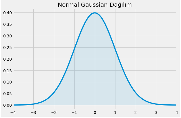
Kaan: Our famous bell curve, or in other words the Normal distribution. Remember that the Gaussian distribution is expressed as

\[\mathcal{N}(\mu, \sigma^2) = \frac{1}{\sigma \sqrt{2\pi}} e^{-(x - \mu)^2 / (2\sigma^2)}.\]

Here $x$ is our random variable, $\mu$ represents the mean, and $\sigma$ represents the standard deviation.

As a shape, what does it look like?

If we visualise it for $\mu = 0$ and $\sigma = 1$, it looks like this:

Then we can express the probability distribution of the error in our problem as

\[\epsilon_i \sim \mathcal{N}(0, \sigma^2).\]

Now, getting back to where we left off, we were thinking about how to calculate each $p(y_i

x_i, \theta)$ in the likelihood expression $L$.

Emre: What does the expression $p(y_i

x_i, \theta)$ tell us?

Kaan: It tells us the likelihood distribution of the random variable $y_i$ given that we know $x_i$ and $\theta$.

We said at the very beginning

\[\hat{y_i} = \theta_0 + \theta_1 x_i + \epsilon_i.\]

Since the only random variables in this equation are $y_i$ and $\epsilon_i$, the distribution of $y_i$ is actually of the same type as the distribution of $\epsilon_i$.

However, we need to pay attention to one thing: while the types of the distributions are the same, the parameter values are different. We can use a property of the Gaussian distribution to find the distribution parameters of $y_i$. If $X \sim \mathcal{N}(\mu, \sigma^2)$ and $Y \sim \mathcal{N}(0, \sigma^2)$, then

\[X = \mu + Y.\]

Using this property, and knowing that $y_i = \theta^T x_i + \epsilon_i$, we can write

\[y_i \sim \mathcal{N}(\theta^T x_i, \sigma^2).\]

This means that the variable $y_i$ also has a Normal distribution with mean $\theta^T x_i$ and variance $\sigma^2$. Thus we can now write the likelihood expression $L$ as the product of the likelihood distributions of the random variables $y_i$:

\[L = \prod_{i=1}^{n} \frac{1}{\sigma \sqrt{2\pi}} e^{-\frac{(y_i - \theta^T x_i)^2}{2\sigma^2}}.\]

Using the property $e^x e^y = e^{x + y}$ of the exponential function, we can rewrite $L$ as

\[L = \left(\frac{1}{\sigma \sqrt{2\pi}}\right)^n e^{-\frac{1}{2\sigma^2} \color{blue}{\sum_{i=1}^{n} (y_i - \theta^T x_i)^2}}.\]

Emre: Why is part of the expression blue?

Kaan: Doesn’t it remind you of something I mentioned above?

Emre: Hmm, the blue part is exactly the “Residual Sum of Squares,” isn’t it?

Kaan: Exactly. So finding the maximum of this likelihood expression is equivalent to finding the point where the RSS—that is, the error—is minimum, right?

Emre: Of course. So in the statistical approach, maximising the likelihood of the data we collected corresponds to minimising the RSS in linear regression.

Kaan: Very good. That is the relationship between the two approaches.

Emre: So where does the Bayesian approach come into play?

Bayesian Inference

Kaan: Since we have started talking in statistical language, we can look at how we reach the Bayesian approach.

Let’s recall Bayes’s rule:

\[p(A | B) = \frac{p(B | A) p(A)}{p(B)}.\]

This rule actually gives us the conditional probability of event $A$ based on observation $B$ (or “evidence,” a term frequently used in Bayesian statistics). In its original form, the denominator of the equation is more complicated, but here we simply wrote $p(B)$ in the denominator. The reason is that when the probability of $A$ is calculated over all probabilities of $B$, the probability of $B$ occurring becomes independent of $A$. This is called “marginalisation.” In this case $p(B)$ acts only as a constant that normalises the equation.

So we can say

\[p(A | B) \propto p(B | A) p(A).\]

Bayes works as follows: In the light of prior information about a hypothesis, we have a preconceived belief (prior); then we obtain some new evidence about the event, and afterwards we reach a posterior belief in the light of the new evidence. That is,

posterior distribution $\propto$ likelihood (information from evidence) × prior distribution (pre-belief)

In summary, in Bayesian statistics the result is basically a probability distribution. That is, instead of point estimates, the probability distributions that make up the estimate! That is, instead of a hypothesis that the parameter of a linear model equals 5, we talk about a parameter that follows a Normal distribution with mean 5 and standard deviation 0.7. Trying to compute point estimates is a “Frequentist” approach. I cannot help mentioning something here. The statistical world is polarised around these two axes. One is the Frequentist approach, which makes little or no use of prior information about the hypothesis, and the other is the Bayesian approach. If you ask any sensible person, “When we get new data about the event we are analysing, do our beliefs get closer to the absolute truth?” they will say “yes.” Understanding this does not require superior intelligence. But what is truly ingenious is setting this up in a mathematical framework that can be expressed under all circumstances. That is what Bayes did. The Bayesian approach handles the prior and the new data within a framework of consistent principles. That is why we are following the Bayesian approach here.

In many cases in the expression above, the likelihood $p(B

A)$ on the right-hand side of the equation is determined by the process that generates the observations. For that process we need to make some assumptions, but let’s not go into that detail. What is most important to note here is that the biggest trick of the Bayesian approach is that the posterior distribution becomes the prior distribution for the next inference. Let’s note this in an important corner of our minds!

Anyway, we have moved too far away from our main problem; let’s take one step back. Based on Bayes’s rule we can now talk about priors and posteriors. In that case, the way to use Bayesian inference in our problem begins with calculating a posterior probability distribution for each parameter.

Nevertheless, if we had a posterior probability distribution for each parameter, we could find the parameter values that maximise the posterior probability (Maximum A Posteriori, MAP, estimation) in order to make predictions. Then we could make the prediction $\hat{y^*}$ as follows:

\[\hat{y^*} = [\text{MAP of } \theta_0] + [\text{MAP of } \theta_1] x^*\]

Here $x^$ represents new observations (new evidence) for which we want to predict $\hat{y^}$.

Kaan: Didn’t something catch your eye here?

Emre: What did I miss?

Kaan: Using MAP estimates would be a “Frequentist” approach. We do not want point estimates. If we are to perform Bayesian inference, we must find the probability distributions of the parameters! For these reasons we should not attach special importance to MAP estimates and should continue on our way.

In that case we have to find a probability distribution for $y^$ for each $x^$. To do that, we need to find the posterior probability distributions of the coefficients in the model—which represent all possible linear models, each corresponding to a different prediction of $y$. Thus each prediction coming from each possible linear model will be weighted by the probabilities of those models. That is,

\[p(y^* | x^*, X, y) = \int_{\theta} p(y^* | x^*, \theta) p(\theta | X, y)\, d\theta.\]

In this formula, we assume that $X$ and $y$ are given to us as the training data. The $x^$ represents new observations. Using these three data pieces we try to predict $y^$. To do that we need to marginalise over the posterior probability distributions of $\theta$. As a result we get a Gaussian distribution whose variance depends on the magnitude of $x^*$.

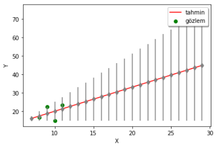
Here another beauty of the Bayesian approach comes to light. If we obtain predictions in this way, we get additional information about the uncertainty of each prediction.

Emre: It is always best to know that you don’t know something!

Kaan: Exactly. As can be seen in the example below, the margin of error for the predictions grows as we move away from the observations (the grey lines show the confidence interval for each prediction). The Bayesian approach thus tells us how confident we can be in our predictions.

In summary, we have looked at the linear-regression problem from both the Frequentist and the Bayesian perspectives.

Advanced Topics

For the more curious: in practice Bayesian inference is often used in parameter-estimation and model-comparison problems. In various types of problems, Bayesian methods yield quite successful results compared with their non-Bayesian rivals (Maximum Likelihood, Regularisation and EM (Expectation-Maximisation)).

Examples of Bayesian inference algorithms include Markov Chain Monte Carlo (more specifically Metropolis–Hastings) and Variational Bayesian Inference. Bayesian techniques are usually used with generative statistical models such as Gaussian Mixture Models (GMM), Factor Analysis and Hidden Markov Models (HMMs). Nevertheless, as we have reviewed above, they are also applicable to linear-regression models.

Real Life

Statistical problems in which Bayesian inference is used range from e-commerce, insurance and sentiment analysis to topic detection in text, finance, healthcare, the stock market and autonomous vehicles. For that reason everyone working in machine learning should learn this subject, even if only at a basic level.

Emre: I think that’s enough. It’s not possible without taking a break :)

Kaan: Okay then, until next time ;)