Emre: How do Apple AirPods cancel noise actively?

Kaan: It’s one of the most enjoyable topics in signal processing. Let’s take a look together to see how it works.

Problem – Active Noise Cancellation

Suppressing unwanted noise acoustically in a specific region is called Active Noise Control. To achieve this, typically one or more loudspeakers emit a signal (anti-noise) with the same amplitude but opposite phase as the noise. The noise and anti-noise sum together in the air and cancel each other out. This happens because two waves of the same amplitude but opposite phase traveling in the same direction physically annihilate each other. We can illustrate this schematically as follows.

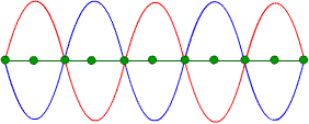
The green points you see in the figure will always be “zero” as a result of the summation (cancellation) occurring in the air.

However, if the phases do not align perfectly, the noise can actually increase!

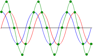
As you can see, this time the green points show a signal with even greater amplitude than the original signal.

So, is generating the inverse of the noise signal really that easy?

Predictably, of course not.

Emre: Why not?

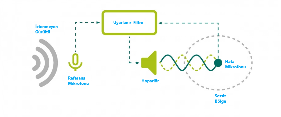
Because the unwanted noise signal never arrives with a fixed amplitude and phase. From the source to the region where we try to cancel the noise, the sound passes through an essentially unknown physical channel (environmental reflections, etc.). Therefore, we need to model this unknown channel. We also need an adaptive filter that keeps track of whether the model is correct—that is, whether the summation in the air truly results in zero. If the model is accurate, we take the signal captured by a reference microphone placed near the source, pass it through that model, invert it, and output it through a loudspeaker placed near an error microphone, thus creating a quiet zone around that microphone.

Thus, an active noise-cancelling system has a block diagram like this:

So what exactly is this adaptive filter? How does it model the air channel mathematically?

Adaptive Filter Design

Basic FIR Filter

Let’s first recall a basic, non-adaptive filter. Assume we have a digital filter whose input is $x(n)$ and output is $y(n)$. The filter has a finite impulse response consisting of $K+1$ taps, and can be written with the following difference equation:

Such filters are called Finite Impulse Response (FIR) filters. This is a deep topic in itself, but for now, what makes these filters attractive are two things: First, they always have linear phase; second, because they have no poles, they are always stable. Explaining why these properties matter would require going into the $z$-domain representation and Fourier transform characteristics of these filters, which is beyond the scope of this post. For now, let’s move on and see how we step from a basic FIR filter toward an adaptive one.

Now, if we think of the above operation as a convolution operation, we can express it as follows (and you can trust me on this, as every textbook says the same—even if I don’t go into every detail here; if you don’t know what this is, it’s worth looking up elsewhere before continuing):

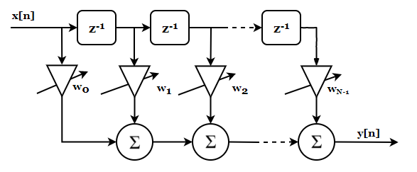
This equation is actually the discrete-time expression of a linear FIR filter. Note that $x$ and $w$ are not multiplied but convolved. The $z$-domain representation of this filter is shown below:

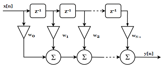
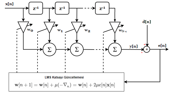
The discrete samples of $x$ are shifted one by one (each $z^{-1}$ block delays its input by one sample, so $x[n]$ goes in, $x[n-1]$ comes out), multiplied by their corresponding weights $w_i$, and all these products are summed. The result is the system output.

So, if we write out the summation explicitly:

That’s all there is to it.

Everything up to here is standard undergraduate-level DSP material—just a refresher or, if you didn’t know it, a foundation.

How do we make this filter adaptive?

Adaptive Filter

Simple: if we change the filter coefficients $w$, we also change the impulse response of the filter, right?

But why would we want to do that?

There are a few interesting reasons. For example, we might want to model an unknown system.

First, we need to imagine that the filter coefficients can change.

Now the $w$ coefficients can change. But according to what rule? When we are modeling an unknown system, what should these coefficients be?

For that, we need an algorithm. By using an appropriate adaptation algorithm, we try to make the adaptive filter resemble the unknown system. Once the error between them becomes zero (or very close to zero), we can say that the filter behaves like the system we wanted to model. At that point, the weights stop changing—unless the unknown system itself changes, in which case the adaptive filter follows suit. Let’s visualize this idea:

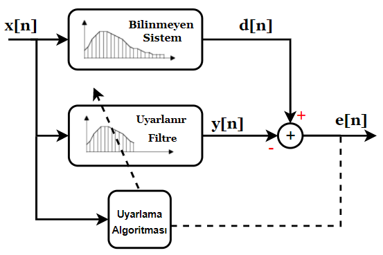
From a mathematical viewpoint, if the adaptation algorithm succeeds in driving the error to zero (it will never reach exactly zero, but can get close enough), the transfer function of the adaptive filter will be equal to that of the unknown system. From that point on, the adaptive filter coefficients no longer update. However, if the unknown system changes over time, the adaptive filter will update itself accordingly.

This is exactly how we model the unknown systems mentioned above in active noise cancellation. You’ll find this idea frequently in other areas: blind deconvolution in image processing, channel estimation in communications, system identification in control, noise reduction or prediction, and so on.

So, what kind of algorithm can drive the error to zero?

Least Squares

The design of adaptive filters is fundamentally rooted in the Least Squares (LS) technique.

This technique is used to solve an over-determined set of linear equations of the form $Ax = b$. The reason is simple: every linear system can be written in that form. Here, $A$ is a matrix, $b$ and $x$ are column vectors. Our goal is to find $x$ given $A$ and $b$.

The size of $A$ is $m \times n$. When $m > n$, we have more equations than unknowns, which means there is only one $x$ that minimizes the error for this set of linear equations.

We can represent this set of linear equations as follows:

Simply put, the solution we seek is the one that minimizes the following

This is equivalent to minimizing the energy of the error vector $\hat{e}$. The double bar $|\cdot|$ denotes the L-2 norm (Euclidean norm, since we square it). We could have used Laplacian or other norms, but that’s not our concern here.

From a geometric perspective, we can also look at the $b$ vector in the column space of $A$. As you can see in the figure below, the $b$ vector is in the null space of $A$ (not in the column space). That is, no combination of the columns of $A$ gives us $b$. However, we can find an approximate solution. The shortest distance between the $b$ vector and the column space of $A$ is our error vector.

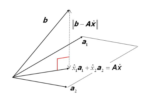
Note: This figure is from the Ordinary Least-Squares presentation.

So, geometrically, the solution is the orthogonal projection of the $b$ vector onto the column space of $A$. When searching for the least squares approximate solution, we are trying to find the set among the column vectors of $A$ that minimizes the error vector, so that the point $A\hat{x}$ is closer to the column space $C(A)$ than any other point. Once we find that point, $\hat{x}_1$ and $\hat{x}_2$ are the solutions to the linear equation set. I hope this gives you some intuition.

Another geometric interpretation is related to the shape of the error performance surface. Plotting $\hat{e}$ with respect to the $n$-dimensional $x$ vector gives us an $n+1$ dimensional hyper-paraboloid. For $x$ with a single dimension, the surface is a simple parabola. In two dimensions, it’s a paraboloid, and it’s impossible to draw for higher dimensions. We actually discussed this paraboloid in the error analysis section of linear regression.

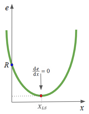
Emre: Where did $R$ come from?

Kaan: Good question. Let’s see where it comes from.

Let’s look at the case where $A$ is a $2 \times 1$ matrix. Then we can calculate the $e$ vector as follows:

Now let’s rename some of the terms in this expression:

If you follow this geometric or linear algebraic solution, you’ll see that the least squares solution comes out as:

As you can see, the parabola in the $e$ error equation intersects the $e$ axis at $R$ where $x$ is zero.

Interestingly, there are other possibilities for the solution of $Ax=b$. If the system is under-determined (more unknowns than equations), then there is no unique solution. Using the singular value decomposition method, a sufficiently good solution can be found.

If the number of unknowns equals the number of equations, then our job is even easier. The solution is directly:

That’s all there is to it.

What does all this have to do with our filter?

We can also express the Finite Impulse Response filter mentioned above in this way.

I hope you see the similarity.

Here, I want to draw your attention to an interesting aspect of engineering. We can look at a problem mathematically from completely different angles. Sometimes we need to try each angle to reach a solution. For example, we wrote the FIR filter as a difference equation, then saw it as a convolution, modeled it in the $z$-domain, and now we write the same equation as a linear system of equations in linear algebra.

Wiener–Hopf Solution and Unknown System Modeling

Now we know how the Least Squares technique solves a set of linear equations. Using this, we can design our adaptive filter.

Earlier, I showed an architecture where the unknown system and the adaptive filter are together. The outputs of the unknown system and the adaptive filter are subtracted to find the error:

What we want to do now is to find the coefficients that minimize this error.

To do this, we need to consider the signals $x[n]$ and $d[n]$ statistically. If $x[n]$ and $d[n]$ are wide-sense stationary and correlated, we can minimize the mean square of the error signal, which is called the Wiener–Hopf solution.

Recall, a random process is wide-sense stationary if its statistics, i.e., mean and autocorrelation function, do not change over time.

Assume the output of the filter (the result of the convolution) is:

To reach the Wiener–Hopf solution, we can square the error $e[n]$; if we take the expected value of both sides, we get the mean squared error (MSE). By minimizing this, we can find the solution.

In this expression, $E{x[n]x^T[n]}$ is the $N \times N$ correlation matrix $\mathbf{R}$, and $E{d[n]x[n]}$ is the $N \times 1$ cross-correlation function $\mathbf{p}$:

Then the mean squared error can be written as:

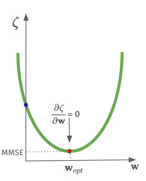
The nice thing is that the above equation is quadratic in $\mathbf{w}$, so it has only one minimum point. Thus, the minimum mean squared error (MMSE) solution ($\mathbf{w}_{opt}$) can be found by setting the gradient (partial derivative) vector to zero:

Yes, you are now looking at the equation that finds the coefficients that minimize the mean squared error!

As you can see, in the Wiener–Hopf solution, there is no feedback! That is, we do not see the error vector in the solution. But in the architecture we drew above, there was feedback in the algorithm that updated the coefficients.

The reason is this: as long as the $\mathbf{R}$ matrix is invertible, the system is stable. Therefore, it is actually sufficient to calculate only the correlation matrix $\mathbf{R}$ and the cross-correlation function $\mathbf{p}$ from $x[n]$ and $d[n]$ to find the optimal filter coefficients.

However, the problem is that for a filter of length $N$ and $M$ samples, calculating $\mathbf{R}$ requires $2 \times M \times N$ multiply-and-accumulate (MAC) operations. Then, inverting $\mathbf{R}$ requires $N^3$ MAC operations, and finally, multiplying by the cross-correlation function requires $N^2$ MAC operations. So, the computational load of the one-shot Wiener–Hopf algorithm is $N^3 + N^2 + 2MN$. Unfortunately, this is too much for real-time applications. Worse, if the statistics of $x$ and $d$ change, the filter coefficients must be recalculated. In other words, the algorithm does not have tracking capability. As a result, Wiener–Hopf is not practical. A similar analysis applies to the Least Squares solution. As the data size increases, the matrix sizes grow. Large matrices make inverting $A$ computationally difficult.

Is there no way out of this?

As always, of course there is.

Real-time systems that want to minimize the error energy use gradient-descent-based adaptive algorithms such as least-mean-squares (LMS) or recursive least squares (RLS).

We mentioned the gradient descent algorithm when talking about Bayesian Inference and Linear Regression.

Least-Mean Squares (LMS)

Let me say this from the start: The LMS algorithm converges to the Wiener–Hopf solution under certain conditions. Here, too, we form the mean squared error performance surface. But this time, instead of the closed-form Wiener–Hopf solution, we use a gradient-descent-based solution.

The summary of the algorithm is this: We start at any point on the hyper-paraboloid, change the filter coefficients in the direction opposite to the steepest gradient, and check whether we have reached convergence. If so, the algorithm ends; if not, we return to the gradient update step.

Recall the gradient of the error performance surface:

In this case, the gradient descent algorithm is as follows:

Here, you see $\mu$ for the first time. Before you ask, $\mu$ is the step size we accept for each gradient calculation. This step size determines the speed of adaptation and the closeness of the steady-state error to the theoretical value (MMSE). By choosing $\mu$ small, we can approach the optimum point with small steps, though convergence will be slow. But if we wander around the optimum point with small steps, the algorithm can be terminated at a point very close to the theoretical optimum. If the step size is large, convergence is fast, but it becomes harder to approach the optimum point due to large jumps.

Anyway, doesn’t something seem off here?

Emre: Of course! We were looking for a new method because calculating $\mathbf{R}$ and $\mathbf{p}$ was too computationally expensive. But this algorithm still depends on them. Isn’t the cost of calculating the performance surface still high?

Kaan: You hit the nail on the head!

We need to find a way to avoid calculating $\mathbf{R}$ and $\mathbf{p}$.

For this, instead of the true gradient, we can use an “instantaneous” gradient estimate! One way to do this is to use only the current value of the error squared when calculating the gradient, instead of the expected value (mean) of the error squared.

Thus, using the instantaneous gradient estimate, the filter update can be written as:

That’s it. Implementing the LMS algorithm is computationally simple. Each step requires $N$ multiply-and-accumulate (MAC) operations to apply the FIR filter, and another $N$ MACs to update the filter.

So, let’s look at the final form of our adaptive filter:

A key stage in algorithm design is deciding on the length of the adaptive filter. Longer filters model the system better, but increase computational load.

The second parameter is the step size. It should be chosen to ensure both fast convergence and algorithm stability. A commonly used selection is:

In this equation, $E{x^2[n]}$ can be interpreted as the power of the input signal.

Let’s summarize the LMS algorithm again:

    \n\\begin{algorithm}\n\\caption{LMS Algorithm}\n\\begin{algorithmic}\n    \\STATE $y[n] = \\sum_{k=0}^{N} w_k x[n-k] = \\mathbf{w}^T\\mathbf{x}[n]$\n    \\STATE $e[n] = d[n] - y[n] = d[n]-\\mathbf{w}^T[n]\\mathbf{x}[n]$\n    \\STATE $\\mathbf{w}[n+1] = \\mathbf{w}[n]+\\mu(-\\nabla_n) = \\mathbf{w}[n] + 2\\mu e[n]\\mathbf{x}[n]$\n\\end{algorithmic}\n\\end{algorithm}\n

Active Noise Cancellation

Now, let’s code the algorithm we defined above and see how active noise cancellation works on a jet engine noise. You can download the jet noise from thebeautybrains.com.

import numpy as np
from scipy.signal import lfilter
from scipy.io import wavfile
import matplotlib.pyplot as plt

# number of iterations
N=10000

# Load the jet noise recording
fs, signal = wavfile.read('insidejet.wav')
y = np.copy(signal)

# Normalize the input signal (8-bit, so divide by 256)
x = np.true_divide(y, 256)

# Create filter coefficients
ind = np.arange(0,2.0,0.2)
p1 = np.array(np.zeros(50)).transpose()
p2 = np.array([np.exp(-(x**2)) for x in ind]).transpose()
p = np.append(p1,p2)
p_normalized = [x/np.sum(p) for x in p]
p_len = len(p_normalized)

# Apply FIR filtering to the input signal
d = lfilter(p, [1.0], x)

# Initialize adaptive filter coefficients
w_len = p_len
w = np.zeros(w_len)

# Find a reasonable step size based on signal power and iteration count (twice 1/(N*E[x^2]))
mu = 2/(N*np.var(x))

error_array = []
# Run the adaptive filter algorithm
for i in range(w_len, N):
  x_ = x[i:i-w_len:-1]
  e = d[i] + np.array(w.T).dot(x_)
  w = w - mu * 2 * x_ * e
  error_array.append(e) 

f1 = plt.figure()
f2 = plt.figure()

ax1 = f1.add_subplot(111)
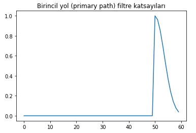
ax1.plot(p)
ax1.set_title('Primary path filter coefficients')
ax2 = f2.add_subplot(111)
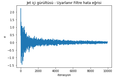
ax2.plot(error_array)
ax2.set_title('Jet noise - Adaptive Filter error curve')
ax2.set(xlabel='iteration', ylabel='e')
plt.show()

When you run this algorithm, the resulting error curve will look like this:

And the primary path filter coefficients we designed will look like this:

Real Life

If you implement the simulations on a Digital Signal Processor (DSP) as they are, you’ll see that it won’t work exactly as in theory. There are two reasons for this. First, the anti-noise emitted by the speaker can acoustically reach the reference microphone and contaminate the signal we measure as reference.

Second, the electrical signal at the output of the adaptive filter passes through another system before it comes out of the speaker, and the error signal also passes through a different system before being read electrically from the microphone and reaching the processor. These problems also need to be taken into account.

In real life, algorithms such as Filtered-x Least Mean Square (Fx-LMS) or Recursive Least Squares (RLS) are used. These algorithms converge faster and require less computational power. If you want to work on this at an advanced level, after this much intuition and theory, you can look into these algorithms as well.

Also, in real-world problems, usually more than one reference microphone and more than one speaker (multi-channel) active noise cancellation systems are developed. The mathematics of multi-channel ANC is not very different from what we have discussed so far. If you understand the basics here, you can easily follow the literature explaining multi-channel solutions.

References

1. Adaptive Filter Theory, Simon Haykin
2. Advanced Topics in Signal Processing, Lecture Notes, Fatih Kara
3. Jet sound recordings
4. What is Column Space? — Example, Intuition & Visualization