Emre: The Markov Chain Monte Carlo method is used everywhere machine learning is needed, from genetics and GPS positioning to nuclear weapons research, RADAR and robotics, and financial forecasting.
Can you explain the intuition behind Markov Chain Monte Carlo (MCMC) without diving into mathematical proofs? Why is MCMC so important?
Kaan: Of course. First of all, let’s start with where this Monte Carlo idea came from.
Problem: What if we can’t compute the posterior analytically?
In the Kalman filter discussion, we were able to compute the posterior analytically. But we may not always be that lucky. In dynamic—time-varying—and nonlinear systems, especially if the distribution is not Gaussian, we may not be able to compute the posterior analytically, and in such cases, advanced techniques like the Monte Carlo method are used. If our model has hundreds or even thousands of parameters, the integral becomes even more intractable.
Emre: Why can’t we compute the posterior analytically?
Kaan: Let’s recall Bayes’ rule:
\[P(\theta|x) = \frac{P(x|\theta) P(\theta)}{P(x)}\]$P(\theta|x)$ gives us the probability distribution of our model parameters given the observations $x$. This is the posterior distribution we want to find. But to compute this, we multiply the prior $P(\theta)$ (the distribution we assume about the parameters before seeing any data) with the likelihood $P(x|\theta)$ (the distribution of the observations if we knew everything about the parameters). This part is easy.
Now, let’s look at the denominator. What was $P(x)$?
Emre: The evidence. That is, the probability that the observations $x$ came from this model, independent of the parameters.
Kaan: Exactly. Here, we need to marginalize over $\theta$. In other words, to leave $x$ alone, we need to integrate over all possible values of $\theta$.
\[Z = P(x) = \int_{\Theta}^{} p(Y|X,\theta)p(\theta)d\theta\]At the end of this integral, we get a normalization constant $Z$. We need this normalization to ensure that the probability values of our posterior distribution range between $0$ and $1$.
But what if we can’t find this integral analytically in closed form?
Emre: We can try to find it approximately.
Kaan: Reasonable. If we could draw samples from the posterior distribution we’re trying to find, maybe we could get an approximate result with a Monte Carlo simulation, but even that wouldn’t be enough because even to do this, we’d have to solve Bayes’ formula and compute the inverse of the distribution to sample from it, which is even harder.
This is where the Markov Chain Monte Carlo algorithm comes in. Simply put, MCMC allows us to draw samples from the posterior distribution without computing the integral or solving the posterior analytically. In this way, we can compute the expected value of the posterior distribution from these samples!
Markov Chain Monte Carlo
MCMC consists of three main components:
- Monte Carlo (MC) approximation
- Markov Chain (MC)
- Metropolis-Hastings (MH) algorithm
Monte Carlo Approximation
In general, the application area of the Monte Carlo method is the estimation of probabilities that are difficult to compute, estimation of parameters resulting from complex systems, obtaining critical values for test statistics, estimation of integrals that are hard to compute, etc. For example, we can estimate the expected value of a statistic whose distribution we cannot express using the Monte Carlo method. We can use the Monte Carlo method to obtain critical values for a statistic whose distribution is unknown or not well-defined. When there are deviations from some assumptions, we can again use the Monte Carlo method to examine the behavior of statistics. More clearly, we can say that the Monte Carlo method can be used to study events we cannot solve analytically.
The early variant of the Monte Carlo approach emerged in the 18th century with the introduction of Buffon’s needle problem. Buffon asked a simple question: “If I randomly drop a needle between parallel lines, what is the probability that the needle will cross at least one of the lines?” Lazzarini used this problem’s solution as a probabilistic method to compute the value of $\pi$. Thus, the solution method became famous.
Actually, the Lazzarini story is a bit complicated. Lazzarini could calculate $\pi$ with great precision using the equation he found, but when the experiment was changed slightly, there was a large deviation, so people wondered if Lazzarini designed the experiment to give the best result. Anyway, that’s outside our topic.
Later, advanced variants of the Monte Carlo method came up again in 1940 at Los Alamos National Laboratory during nuclear weapons research. As the algorithm gained popularity, it began to be used in every field today, from genetics and GPS positioning to RADAR, robotics, and financial forecasting.
So what made the Monte Carlo method so special or successful?
The secret behind the Monte Carlo method’s success is actually the Law of Large Numbers (LLN) that we know from probability theory. In probability theory, the LLN is a theorem that describes the result of repeating the same experiment a large number of times. According to the LLN, the average of the results from a large number of trials should be close to the expected value, and as we do more trials, it should get even closer. For example, consider a process with random outputs. Observe a random variable many times. Then, the average of the observed values will stabilize in the long run. Thus, the best way to estimate the expected value of a random variable is to use the sample average from a sufficiently large number of observations as an unbiased estimator of the expected value. That’s the main idea.
As a result, the MC component allows us to draw samples from a distribution (e.g., $\theta_t \sim \mathcal{N}(0.5, \sigma^2)$) and compute the expected value of the distribution from these samples.
Remember, the advantage of the MC step is this seemingly simple but very functional LLN assumption. I’ll get to why it works.
Importance Sampling
The next step, in the sequence of ideas leading to Markov Chain Monte Carlo, is “importance sampling” (there are even earlier ideas, but I won’t go into that much detail).
Our goal is to find a way to estimate $P(x)$ or $Z$ (the integral above) approximately. Now we have the LLN idea from the MC approach. Let’s see what else we can add.
The essence of this idea is: we propose a distribution $q(\theta)$ that we know and think is close to the posterior distribution of the actual system we’re working on, and we use this distribution as follows:
\[Z = \int_{}^{} \frac{p(Y|\theta)p(\theta)\color{red}{q(\theta)}d\theta}{\color{red}{q(\theta)}}\]After all, dividing the numerator and denominator by the same thing doesn’t change the result, right?
In this case, we can write $Z$ as:
So $W$ here is a function of $\theta$. For example, suppose we draw samples from $q(\theta) \sim \mathcal{N}{(0, 1000)}$, we can substitute the values and compute $W$. Here, again, the LLN helps us. The Law of Large Numbers tells us:
\[Z \approx \frac{1}{N} \sum_{i=1}^{N} W(\theta^{(i)})\]This means that if $W$ is a function of $\theta$, this integral is equivalent to the average of the samples (I won’t go into the proof).
So, using the samples from our $q(\theta)$, we can now approximately compute $Z$. Nice, so the problem should be solved now, right?
Emre: The question suggests otherwise.
Kaan: Yes. Unfortunately, the problem is that to plot histograms of the posterior distribution with this $Z$ calculation, we need $N^K$ samples for $K$-dimensional ($K$ random multivariate) problems. In a real-world problem where $N$ is a million and $K$ is $25$, ($10^{150}$ samples needed), the histograms will require so much computation that they can’t be calculated in a reasonable time. This is called the curse of dimensionality.
Emre: There’s a way out of this too, right?
Kaan: Of course. Drawing samples from a proposed distribution gave us a new perspective. Now, by drawing samples from a proposed distribution and using the LLN, we’ve learned to make estimates. But to solve high-dimensional estimation problems, we need to look at the problem from a completely different angle instead of computing histograms.
Instead of histograms, we can work on predictive distributions.
Given past data $Y_{1:t}$, we can write the probability distribution for our future prediction $Y_{t+1}$ at time $X_{t+1}$ as:
\[P(Y_{t+1}|X_{t+1},Y_{1:t}) = \frac{1}{Z} \int_{}^{} P(Y_{t+1}|X_{t+1}, \theta) P(Y_{t+1}|\theta)P(\theta)d\theta\]We know how to find $Z$ with Monte Carlo importance sampling. But this time, we need to do something more.
We’re about to do one of the most important mathematical tricks that makes importance sampling useful!
We’ll use the $W$ trick again (i.e., multiply and divide by $q(\theta)$ to make $W$ a function of $\theta$), but this time we’ll apply Monte Carlo to both the numerator and the denominator “at the same time”!
Then, we can express our predictive distribution as:
\[P(Y_{t+1}|X_{t+1},D) = \sum_{i=1}^{N} \hat{w}(\theta^{(i)})P(Y_{t+1}|X_{t+1},\theta^{(i)})\]where
\[\hat{w}^i = \frac{w^i}{\sum_{j}^{}w^j}\]Here, we’re again computing a histogram, but this time the weights are normalized. As a result, the integral of the distribution we compute will be $1$. That is, it will satisfy the necessary condition for being a probability distribution function.
We’ve made a big leap forward. The derivation from the initial form of the predictive distribution to here is too long and complex to do here.
But let me explain the logic. By applying Monte Carlo to both the numerator and the denominator at the same time, we got rid of $Z$. We no longer have to compute it. This derivation is the most important derivation in Bayesian inference. If you plan to do a PhD in these topics, you must prove this derivation to yourself.
Now, without having to compute histograms for huge-dimensional data, we can compute the approximate posterior distribution. However, unfortunately, this doesn’t solve all our problems.
Importance sampling can be used for problems with $5$-$10$ parameters (e.g., bioinformatics, logistic regression). As long as the $q(\theta)$ we propose is a reasonable distribution and contains the expected value of $\theta$, we can trust this approach. In robotics problems (e.g., autonomous vacuum robots), the Sequential Importance Sampling variant called Particle Filtering is often used.
However, as the number of parameters to estimate increases, the $q(\theta)$ distributions we propose inevitably become unrealistic. Therefore, for cases with a high number of parameters (e.g., financial forecasting), another solution was needed. Thus, the Markov Chain Monte Carlo algorithm was born.
Markov Chain (MC)
A Markov chain ensures that the state $\theta$ depends only on $\theta_{t-1}$. That is, if you model a stochastic state-space model as a Markov process, the next state of the system is conditional only on the previous state $\theta_{t-1}$, not on all previous states $\theta_{t-1, t-2, …, t-N}$.
We can express the new state as: $\theta_{t} \sim \mathcal{N}(\theta_{t-1}, \sigma^2)$.
That is, we produce a new random sample by using the previous random sample as the mean of the distribution. We can visualize this as follows:
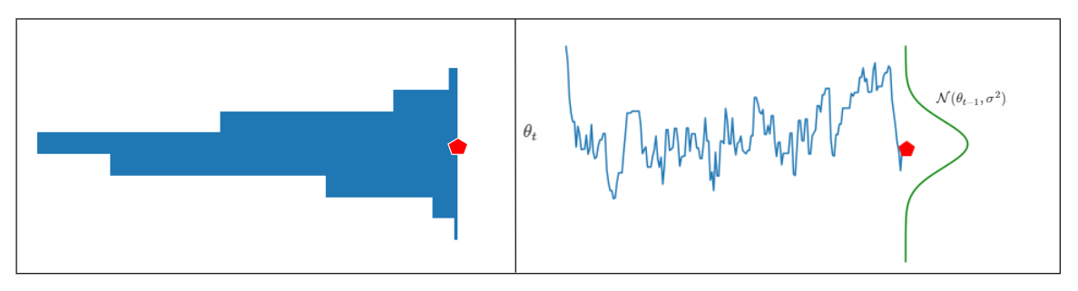
What does this figure show us?
On the right, each new sample is generated from a Normal distribution whose mean is the previous sample. The histogram on the left is the histogram of the generated random samples. Notice that the histogram doesn’t look much like the proposal distribution on the right. That’s because these samples are produced by random-walk.
As a result, we still manage to draw samples from a stationary (even ergodic) distribution using the Markov chain. Still, the distribution of the samples we draw doesn’t look like the posterior (or the proposal distribution). The Metropolis-Hastings algorithm will solve this problem.
Let me mention that here we assumed the Markov Chain has a stationary distribution and is an ergodic process. The chain must have many properties (irreducibility, periodicity, recurrence, etc.). This is a crucial point of MCMC and could be discussed for pages, so for now, trust me that this assumption works.
Emre: At least, what does “ergodic” mean?
Kaan: Let’s call the probability matrix that defines the transitions between states in the Markov Chain $T$. If all states in the $T$ transition matrix can reach each other and the average time (number of samples) we take is long enough, this chain is called an ergodic Markov chain. If the average time is long enough, theoretically, the sample average will approach the true mean of the signal.
Metropolis-Hastings (MH) algorithm
This step determines which of the samples produced by the Markov chain from the proposal distribution we accept and which we reject.
First, we find the ratio of the probability that the newly drawn (current) sample from the Markov chain came from the posterior to the probability that the previous sample came from the posterior:
\[r=min\{1,\frac{likelihood\ of\ proposed\ sample \times prior\ probability\ of\ proposed\ sample}{likelihood\ of\ previous\ sample \times prior\ probability\ of\ previous\ sample}\}\]If $r=1$, we immediately accept the proposed sample. This means the probability that the new sample belongs to the posterior is obviously higher. But if this ratio is less than $1$, we have a choice.
If the ratio is less than $1$, we compare this ratio to a random number drawn from the uniform distribution $U[0,1]$ and decide whether to accept the new sample from the Markov chain.
If the random number from the uniform distribution is less than our acceptance probability ($r$), we accept the new sample $x^{\star}$ as the new sample; otherwise, our new sample is the same as the previous one.
I can try to explain this with an analogy. I pose a problem and actually have a solution in hand. A new answer comes from somewhere to the question I posed. If the solution in this answer is better than the one I have, I accept the new answer as the current solution; otherwise, I reject it and keep the old solution; if I’m not sure, I roll the dice whether to accept it or not!
MCMC Algorithm
Let’s review the chain of ideas that brought us to the MCMC method. First, we looked at the Monte Carlo approximation. For cases where we couldn’t compute integrals, we used the Law of Large Numbers and developed the importance sampling method. But we saw that computing histograms is computationally expensive (in neural networks, thousands of dimensional variables are computed; as the number of dimensions increases, this method becomes computationally impractical). We decided to proceed via predictive equations. Instead of approximately finding $Z$, we moved to the normalized importance sampling method, which applies Monte Carlo to both the numerator and denominator at the same time and gets rid of computing $Z$. We also saw that this method works for problems with few parameters. As the number of parameters increases, our assumptions about the proposed distribution move away from reality and become unrealistic. Therefore, we needed a new method that would work for many parameters.
Now we can look at the Metropolis-Hastings algorithm of MCMC and how well it works.
Assuming $X$ is our state vector (the “state” in the state-space model) and $q$ is the proposal distribution, we can write the MCMC algorithm as follows:
In step 1, we initialize our parameter vector and choose the proposal distribution that we think resembles the target distribution. In step 2, we start a loop. In step 3, we draw a random number from the uniform $U$ distribution in $[0,1]$. In step 4, we pass our $x^{i}$ sample through the proposal distribution $q$. That is, we draw a sample from $q$ with mean $x^{i}$. In other words, $x^{\star} = X^{(i)} + \mathcal{N}(0, \sigma^2)$. (Our new sample will come out somewhere near the previous one.) In step 5, we compute the ratio of the posterior of the new parameter to the posterior of the previous parameter. This ratio determines our “acceptance probability.” Notice that I deliberately wrote $Z$ without canceling it. In fact, at this step, the $Z$s cancel, so we no longer need to compute that infamous integral! In step 6, we compare this ratio to the sample we drew from the uniform distribution. If the random number from the uniform distribution is less than our acceptance probability ($r$), we accept the new sample from the Markov chain as the new sample $x^{\star}$; otherwise, our new sample is the same as the previous one. In step 7, we check if we’ve reached the end of the loop; if not, we increment the counter and go back to step 3.
We can visualize the flow of the algorithm as follows:
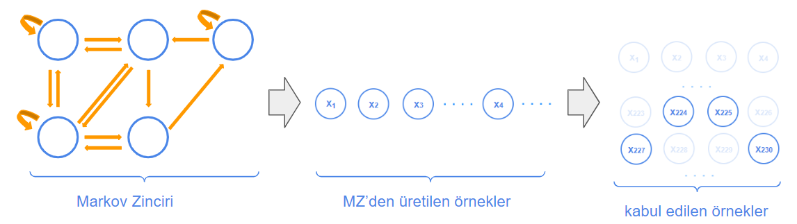
The figure on the left shows us our Markov Chain.
In MCMC, we accept some samples from the Markov Chain (which we assume is ergodic) that meet our criteria. To see interactively how MCMC reaches the target distribution by making these selections, you can check out The Markov-chain Monte Carlo Interactive Gallery.
Coding the Algorithm
Now we need to define a model. For simplicity, let’s assume the target distribution (likelihood) is a Normal distribution. As you know, the Normal distribution has two parameters: the mean $\mu$ and the standard deviation $\sigma$. For convenience, let’s take $\sigma=1$ and try to infer the posterior distribution of $\mu$. For every parameter we want to infer, we also need to assume a prior distribution. Let’s also assume this is a Normal distribution for convenience. So our assumptions are as follows:
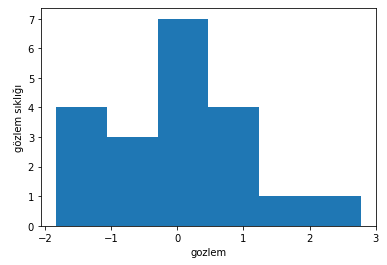
Let’s generate $20$ random observations from a Normal distribution with mean $0$. You can think of these as coming from the system we observe in real life.
import numpy as np
import pandas as pd
import scipy as sp
import matplotlib.pyplot as plt
from scipy.stats import norm

np.random.seed(225)

data = np.random.randn(20)
plt.hist(data, bins='auto')
plt.xlabel('observation')
plt.ylabel('frequency')
plt.show()
The histogram of the generated random observations will look like this:
The nice thing about this model is that we can now also compute the posterior analytically. If the likelihood is a Normal distribution with known standard deviation, then a Normal prior for $\mu$ will be conjugate (i.e., the prior and posterior distributions will be the same type). You can find how to compute the parameters of the posterior from Wikipedia or elsewhere. The mathematical derivation can be found here.
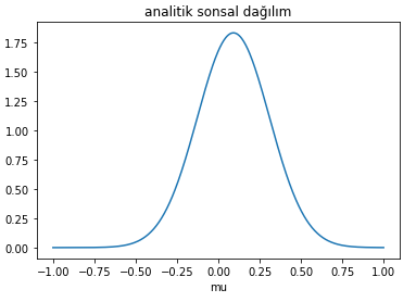
Let’s see what the analytical posterior looks like when we have the observations.
def compute_posterior_analytical(obs, x, mu_init, sigma_init):
    sigma = 1.
    n = len(obs)
    mu_post = (mu_init / sigma_init**2 + obs.sum() / sigma**2) / (1. / sigma_init**2 + n / sigma**2)
    sigma_post = (1. / sigma_init**2 + n / sigma**2)**-1
    return norm(mu_post, np.sqrt(sigma_post)).pdf(x)

x = np.linspace(-1, 1, 500)
posterior_analytical = compute_posterior_analytical(data, x, 0., 1.)
plt.plot(x, posterior_analytical)
plt.xlabel('mu')
plt.title('analytical posterior distribution')
plt.show()
The probability distribution of $\mu$ (analytically) based on our observations looks like this:
In real life, we’re not that lucky. Usually, the prior isn’t conjugate and the posterior isn’t easy enough to derive by hand. So, it’s time to bring in the MCMC algorithm.
The first step of the algorithm was to initialize the parameter we want to find the distribution of. This is something we can do using all the information we have about the parameter. Let’s assume we have a hunch that the $\mu$ parameter we’re trying to find will be around $1$. We can use this by initializing $\mu = 1$.
From this starting point, we need to jump to another point (this is where the Markov component comes in). But where?
We can be quite sophisticated here or act naively. This is where we need the proposal distribution I mentioned earlier. We’ll jump to the next point according to this proposal distribution. In this sense, the Metropolis sampler is actually naive. It jumps to a new point according to a Normal distribution centered at the current $\mu$ value, and this Normal distribution has nothing to do with the model distributions we assumed earlier. How far we can jump depends on the width (standard deviation) of this proposal distribution.
What do we do in the next step?
Emre: We check whether to accept the new point we’ve reached.
Kaan: Very good.
If the new Normal distribution at the point we reach explains the observations better, we accept this new point. But what does “explains better” mean?
That is, we compute the probability of the observations using the proposed $\mu$ and standard deviation. We act a bit like a hill climbing algorithm. We propose jumps in random directions, and if the likelihood of the proposal is higher than the current likelihood, we accept the jump. Eventually, we’ll reach the place where $\mu = 0$ and can’t jump anywhere else. But since we want to have a distribution in the end, we’ll sometimes accept points far from $0$. When accepting, we divide the likelihood of the proposal by the likelihood of the current point. We look at the resulting ratio to decide whether to accept.
Now let’s look at the MCMC code and what results it produces.
N = 100000
mu_current = 1.0
prior_mu = 1.0
prior_sd = 1.0
proposal_sd = 0.2
posterior = [mu_current]
accept_count = 0
for i in range(N):
    # propose new position
    mu_proposal = norm(mu_current, proposal_sd).rvs()

    # compute likelihood (multiply probabilities for each observation)
    likelihood_current = norm(mu_current, 1).pdf(data).prod()
    likelihood_proposal = norm(mu_proposal, 1).pdf(data).prod()

    # compute prior probabilities for current and proposed mu
    prior_current = norm(prior_mu, prior_sd).pdf(mu_current)
    prior_proposal = norm(prior_mu, prior_sd).pdf(mu_proposal)

    p_current = likelihood_current * prior_current
    p_proposal = likelihood_proposal * prior_proposal

    u = np.random.uniform()

    # compute acceptance probability
    r = p_proposal / p_current

    # accept?
    if u < r:
        # update position
        mu_current = mu_proposal
        accept_count += 1

    posterior.append(mu_current)

print("Efficiency = ", accept_count/N)
When you run this algorithm, you’ll start to see results like this:
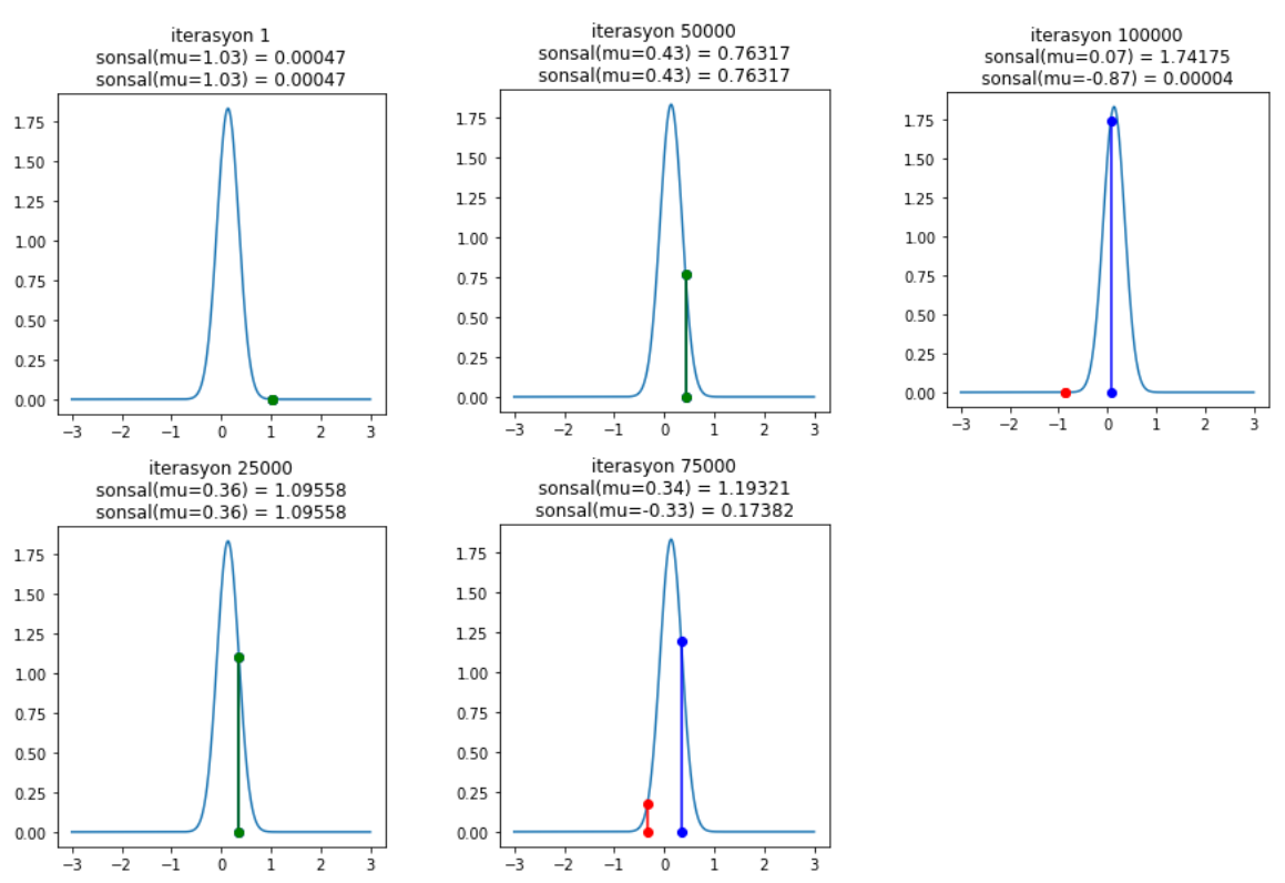
Pay attention to how proposed positions are rejected at the $75{,}000$th and $100{,}000$th iterations. To avoid clutter, we plot every $25{,}000$ steps, but you can examine how acceptance/rejection works at each step if you want. As a result, MCMC finds the posterior distribution and shows that the highest probability is around $\mu = 0$.
At the end of the simulation, the efficiency we compute shows how many of the proposed samples were accepted. If more than 70% are accepted, our model is set up correctly. In this simulation, the acceptance rate is around 72%, which shows we’re on the right track.
Let’s compare the posterior distribution we obtained with MCMC to the analytical distribution.
import seaborn as sns

ax = plt.subplot()
sns.distplot(np.array(posterior[500:]), ax=ax, label='posterior estimate')
x = np.linspace(-1.0, 1.0, 500)
post = compute_posterior_analytical(data, x, 0, 1)
ax.plot(x, post, 'g', label='analytical posterior')
_ = ax.set(xlabel='mu', ylabel='credibility (belief)');
ax.legend();
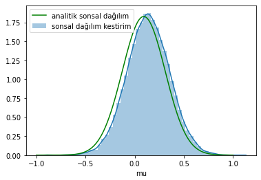
We calculated the histogram of the $\mu$ values we accepted. Don’t let this confuse you. The distribution we found also looks like the distribution of the observations sampled from the Normal distribution, but this is our estimate. In another model, a completely different distribution could have emerged.
Real Life
MCMC has two well-known problems.
- Dependence on initial values
To get rid of the first problem, we can discard the first samples we draw (e.g., the first 500) until the chain stabilizes.
- Autocorrelation of the Markov Chain
For the Markov process to work as expected, a state should depend only on the previous state. As dependence on earlier states increases, MCMC’s performance will decrease.
Let’s look at the autocorrelation of the posterior distribution we obtained.
from pymc3.stats import autocorr
lags = np.arange(1, 30)
plt.plot(lags, [autocorr(np.array(posterior), l) for l in lags])
plt.xlabel('lag')
plt.ylabel('autocorrelation')
plt.title('analytical posterior distribution')
plt.show()
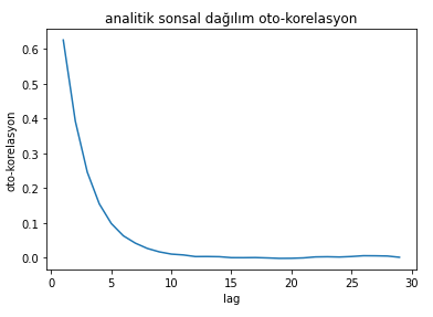
As you can see from the figure, the $i+1$th sample is not only dependent on the $i$th sample. There is also strong correlation with earlier samples. To get rid of this problem, instead of accepting consecutive samples, we can accept every $n$th sample. This is called “thinning” in the Markov Chain literature. The sample space is enlarged, and every $n$th sample is kept.
As a result, by using MCMC, we can obtain:
- the posterior distribution of model parameters
- the posterior distribution of predictions
- the posterior distribution for model comparison
Other than these two problems, Metropolis-Hastings has its own issues. For example, the proposal distribution chosen by MH is symmetric. The Gibbs Sampler is another MCMC variant introduced to automate this choice.
On the other hand, MCMC is computationally intensive. That’s why you may find studies in the literature that parallelize the algorithm.
There’s also the Hamiltonian Monte Carlo variant, which makes smarter jumps by looking at the proposals. You can check that out too.
References
- Machine Learning: A Probabilistic Perspective, Kevin P. Murphy
- Approximate Inference using MCMC, Ruslan Salakhutdinov
- Monte Carlo Methods, Sinan Yıldırım
- Importance sampling & Markov chain Monte Carlo (MCMC), Lecture Notes, Nando de Freitas