Machine Learning 5 - Kalman Filter Based Autonomous Driving

08 Mar 2020

Reading time ~20 minutes

Emre: What is the logic behind the Kalman filter? How does it work in so many fields, from autonomous robots to the Apollo space program?!

Kaan: Good question. Essentially, the Kalman filter is a fascinating algorithm discovered by Hungarian-American mathematical system theorist Rudolf Kalman, and it has been used since the 1960s and is still widely applied today.

The Kalman filter is one of the most important algorithms discovered in the twentieth century, and every signal processing or machine learning expert who works with sensors and makes predictions from sensor data should know why.

Let me try to explain with an example.

Problem - Designing an Autonomous Vehicle

Let’s assume we are designing a self-driving (autonomous) car. We can assume our car has many sensors to detect other cars, pedestrians, and cyclists. Knowing the location of these objects helps the vehicle make decisions and avoid collisions. However, besides knowing the location of objects, the autopilot must also predict its own and other vehicles’ future positions to plan ahead and avoid accidents.

So, the autopilot should have not only sensors to determine the positions of objects but also mathematical models to predict their future positions. In the real world, prediction models and sensors are not perfect. There is always uncertainty. For example, weather conditions can affect sound sensor data (increasing uncertainty), so the vehicle cannot fully trust the data from these sensors. Our goal is to reduce this uncertainty and strengthen our predictions using Kalman filters!

Before going into the theory in detail, let me note that to understand Kalman well, you need a strong background in linear dynamic systems, state-space, matrices, Markov chains, and covariance.

Emre: Can you provide reference sources?

Kaan: Of course, linear dynamic systems and state-space models are taught in Control Theory courses, matrices in Linear Algebra courses, and finally Markov Chains and Covariance in Probability and Statistics courses.

Kalman Filter

The mathematics of the Kalman filter can be intimidating in many places you find on Google, but I will try to explain it simply here.

Let’s start by building our mathematical model.

Let’s assume our autopilot has a state vector $\vec{x}$ representing position ($p$) and velocity ($v$):

$$ \vec{x} = \begin{bmatrix} p\\ v \end{bmatrix} $$

Remember, the state vector is just a list of numbers related to your system’s basic configuration; it can be any combination of data. In our example, we took position and velocity, but it could also be the amount of fuel in the tank, engine temperature, the position of a user’s finger on a touch surface, or any other sensor data we need to track.

Let’s also assume our car has a GPS sensor with about 15 meters of accuracy. Actually, 15 meters is quite good, but to detect a crash in advance, we need to know the vehicle’s position much more precisely. So, in our scenario, let’s assume GPS data alone is not enough. If we were thinking about a home-cleaning robot, accuracy would be even more important, but the solution would not be very different.

An important part of modeling is thinking about the physical phenomenon. For example, the autopilot knows something about how the car moves. It knows the commands sent to the engine or steering, and if it is moving in a direction and nothing gets in the way, it will probably continue in that direction in the next moment. But of course, it cannot know everything about the actual movement. The car can be pushed by strong wind, the wheels may slip a bit due to the ground, or it may turn unexpectedly on rough terrain. So, the amount the wheels turn may not exactly show how much the car actually traveled, and in this case, the autopilot’s new position estimate based on previous positions will not be perfect.

The GPS “sensor” also gives us a new state (position and velocity) only indirectly and with some uncertainty or errors.

Can we use both pieces of information to make a better estimate than either could give us alone?

Let’s visualize this a bit.

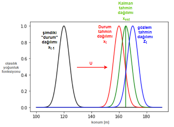
Notice that we do not know the “true” position and velocity. Therefore, even the position of the state at $x_{t-1}$ is shown as a probability distribution (prior distribution), and we think the vehicle is most likely at the expected value ($\mu$) of this distribution. The $U$ in the figure represents the control variable vector, which includes the acceleration/deceleration commands sent to the engine within the autopilot’s knowledge; the red distribution is the expected value $x_t$ of the state prediction equations, and the blue distribution is the expected value $z_t$ of the measurement prediction equations. The Kalman filter multiplies the state prediction probability distribution and the measurement prediction probability distribution to find a new distribution. The expected value of this distribution, $x_{est}$, is our new estimate of the vehicle’s state (position + velocity), which is actually better than either estimate alone (i.e., the variance of the state prediction and measurement prediction distributions is reduced, and the expected value is the optimal estimate).

Now let’s get a bit more into the mathematics. We can set up the state vector prediction equation as follows:

$$ \begin{equation} \begin{split} \color{red}{\mathbf{\hat{x}}_t} &= \mathbf{A} \mathbf{\hat{x}}_{t-1} + \mathbf{B} \color{red}{\vec{\mathbf{u}_t} + \varepsilon_{x}} \end{split} \end{equation} $$

$\varepsilon_{x}$ is an error distribution modeling the uncertainty in our state vector estimate, and in the Kalman filter, this distribution is always assumed to be Gaussian. Notice that our prediction is actually set up as a linear equation. $A$ and $B$ are the linear system matrices in this dynamic equation, representing the state vector $\hat{x}_{t-1}$ and the control (external factor) vector $\vec{u_t}$.

Emre: What does it mean to multiply a distribution by a coefficient matrix in linear systems?

Kaan: It would be better if I showed this visually.

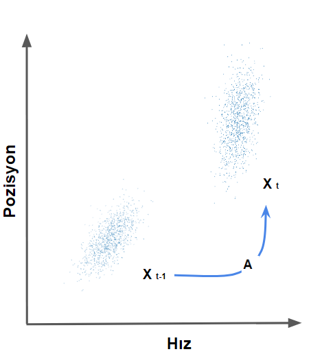
The multiplied matrix takes every point in the original distribution and moves it to a new place, which, if our model is correct, represents the stochastic conditions the system will be in at the next time step. By “state” here, we mean the physical position and velocity of the system, because our state vector represents these two parameters. After multiplying by the $A$ matrix, I will talk about what happens to the variance and covariance soon. For now, just see that this multiplication changes the covariance matrix of the new state vector.

One more point: in systems not controlled externally, the control vector ($\vec{u}$) and control matrix $B$ are ignored.

The predicted state estimate is also called the prior estimate because it is calculated before the measurement is taken.

Let’s look at the measurement prediction equation:

$$ \begin{equation} \begin{split} \color{royalblue}{\mathbf{\hat{z}}_t} &= \mathbf{C} \color{red}{\mathbf{\hat{x}}_{t}} + \color{darkorange}{\varepsilon_{z}} \end{split} \end{equation} $$

Here, $C$ is again the coefficient of the linear prediction equation. Notice that the state vector prediction is used as input in the measurement prediction, and we add the measurement error probability distribution $\varepsilon_{z}$ to the equation. Soon it will be clear why we do this. For now, it’s enough to say that this error distribution is also assumed to be Gaussian.

So how does the Kalman filter use these two predictions to make a reliable $x_{est}$ state vector estimate (Kalman estimate)?

We can show it like this:

$$ \begin{equation} \begin{split} \color{yellowgreen}{\mathbf{x}_{est}} &= \color{red}{\mathbf{\hat{x}}_{t}} + \mathbf{K} (\color{royalblue}{\mathbf{z}_t} - \color{royalblue}{\mathbf{\hat{z}}_t}) \end{split} \end{equation} $$

Yes, this is the secret. This is called the posterior estimate, and $K$ is the term known as the Kalman gain in the literature. The $z_t - \hat{z}_t$ inside the parentheses is called the correction term. So what does all this mean?

This equation tells us: we have a new state vector estimate $\hat{x}_t$ and a new position estimate (measurement prediction) $\hat{z}_t$ from the sensor. If our measurement prediction matches the observation, the expression inside the parentheses will be zero. So we can trust our state vector estimate. When the difference is greater than zero, our state vector estimate needs a correction from the observation. The difference between the observation and our measurement prediction is a measure of this correction. How much of this difference we take into account is determined by the Kalman gain $K$. The Kalman gain is a measure of the new information. If the information expressed by this difference is large, the gain will be high, i.e., its weight will increase; otherwise, it will be small.

Kalman does something nice here; who would want to use a highly uncertain estimate with high weight in another estimate?

Linear Dynamic System Model

At this point, it’s time to calculate the linear dynamic system coefficients ($A,B,C$) in the prediction equations we set up above. Now, to model our linear dynamic system, we can explicitly write the motion equations for our autonomous vehicle.

Remember, we defined our state vector as:

$$ \vec{x} = \begin{bmatrix} p\\ v \end{bmatrix} $$

Using this model and assuming the GPS only reports position $p$, we can calculate $A,B$, and $C$ using the general motion equations for position and velocity:

$$ \begin{split} \color{deeppink}{p_t} &= \color{royalblue}{p_{t-1}} + {t} &\color{royalblue}{v_{t-1}} + &\frac{1}{2} \color{darkorange}{a}_t {t}^2 \\ \color{deeppink}{v_t} &= &\color{royalblue}{v_{t-1}} + & \color{darkorange}{a}_t {t} \end{split} $$

We can write this in matrix form as:

$$ \begin{align} \color{deeppink}{\mathbf{\hat{x}}_t} &= \begin{bmatrix} 1 & t \\ 0 & 1 \end{bmatrix} \begin{bmatrix} p_{t-1}\\ v_{t-1} \end{bmatrix} + \begin{bmatrix} t^2/2\\ t \end{bmatrix} a_t + \color{darkorange}{\varepsilon_{t}} \end{align} $$

We modeled our measurement prediction as:

$$ \begin{equation} \begin{split} \color{royalblue}{\mathbf{\hat{z}}_t} &= \mathbf{C} \color{red}{\mathbf{\hat{x}}_{t}} + \color{darkorange}{\varepsilon_{z}} \end{split} \end{equation} $$

Assuming the GPS sensor only gives us position $p$:

$$ \begin{align} \color{royalblue}{\mathbf{\hat{z}}_t} &= \begin{bmatrix} 1 & 0 \end{bmatrix} \begin{bmatrix} p_{t}\\ v_{t} \end{bmatrix} + \color{darkorange}{\varepsilon_{z}} \end{align} $$

So now we know $A$, $B$, and $C$:

$$ \begin{align} A &= \begin{bmatrix} 1 & t \\ 0 & 1 \end{bmatrix}\\ B &= \begin{bmatrix} t^2/2 \\ t \end{bmatrix} \\ C &= \begin{bmatrix} 1 & 0 \end{bmatrix} \end{align} $$

Kalman Filter Algorithm

The Kalman filter recursively repeats two steps: prediction and update with information from the measurement. A prediction is made with the available information, and then a correction update is made with the information from the measurement. The resulting posterior distribution is used as the prior distribution in the next step. Thus, our prior beliefs are updated.

A small note from the Bayesian philosophy: it turns out that not being prejudiced, but being able to change your judgment when new information comes, is a big advantage!

Prediction

Let’s start by calculating the variance and covariance.

First, let’s write the variances of the distributions we use in the state vector and measurement predictions:

$$ \begin{equation} \begin{aligned} \color{darkorange}{\varepsilon_{x}} = \mathbf{E}_x &= \begin{bmatrix} \Sigma_{pp} & \Sigma_{pv} \\ \Sigma_{vp} & \Sigma_{vv} \\ \end{bmatrix} \\ \color{darkorange}{\varepsilon_{z}} = \mathbf{E}_z &= \sigma_{z}^2 \end{aligned} \end{equation} $$

Since there is more than one random variable in the state vector, $E_x$ is actually a covariance; on the other hand, since there is only one random variable in the measurement vector, $E_z$ represents the variance of that variable.

Using this information, we can express the covariance we get for the state vector prediction as:

$$ \begin{equation} \begin{split} \color{red}{\mathbf{\hat{\Sigma}_{t}}} = \mathbf{A} \mathbf{\Sigma_{t-1}} \mathbf{A}^T + \color{darkorange}{\mathbf{E}_x} \end{split} \end{equation} $$

Derivation

This derivation is not that difficult. If we express the covariance of $x$ as:

$$ Cov(x) = \Sigma $$

and we know in the prediction equation that $A\hat{x}_{t-1}$ is present, we can express the covariance after multiplying the random variable by a constant as:

$$ \begin{equation} \begin{split} Cov(\color{firebrick}{\mathbf{A}}x) &= \color{firebrick}{\mathbf{A}} \Sigma \color{firebrick}{\mathbf{A}}^T \end{split} \end{equation} $$

Emre: What happened to $B$ and $u$?

Kaan: $u$ is not a random variable; we know what it is. So we do not talk about its variance. Like the variance of a constant, we take its variance as zero and ignore it.

This is actually a derivation we know from classical probability theory.

Anyway, in summary, what we do in this expression is: we calculate the prior covariance, $\mathbf{\Sigma_{t-1}}$, and add the expected variance of our state vector. This gives us our predicted covariance.

At this point, we now have prediction equations, and we can calculate the $A$ and $B$ coefficients from the linear dynamic system we assumed.

$$ \begin{equation} \begin{split} \color{red}{\mathbf{\hat{x}}_t} &= \mathbf{A} \mathbf{\hat{x}}_{t-1} + \mathbf{B} \color{red}{\vec{\mathbf{u}_t} + \varepsilon_{x}} \end{split} \end{equation} $$

$$ \begin{equation} \begin{split} \color{red}{\mathbf{\hat{\Sigma}_{t}}} = \mathbf{A} \mathbf{\Sigma_{t-1}} \mathbf{A}^T + \color{darkorange}{\mathbf{E}_x} \end{split} \end{equation} $$

Correction (Update) After Measurement

The Kalman filter also takes into account that our sensors are not perfect. The variance of the error from the measurement enters into the calculation of the Kalman gain and thus plays a role in our latest estimate.

Now we need to use the variances of the state vector and measurement vector predictions to calculate the Kalman gain $K$.

So how is the Kalman gain calculated?

This is a bit more complicated. The general idea to remember is: the higher the variance (uncertainty) of the measurement error, the smaller the Kalman gain should be so that the difference between our measurement prediction and the actual observation does not affect our state vector estimate with too high a weight.

Without going into the proof, we can express the Kalman gain as:

$$ \begin{equation} \color{red}{\mathbf{K}_t} = \color{red}{\mathbf{\hat{\Sigma}_t} \color{black}{\mathbf{C}^T} (\color{black}{\mathbf{C}} \color{red}{\mathbf{\hat{\Sigma}_t}} \color{black}{\mathbf{C}^T}} + \color{darkorange}{\mathbf{E}_z})^{-1} \end{equation} $$

Don’t let this expression scare you. We multiply some matrices, but what actually happens is: we multiply the inverse of the matrix product that includes the measurement error variance by the covariance estimate. Since we take the inverse, as the variance in the measurement increases, the value of this product decreases. As a result, the higher the variance in the measurement, the less information our measurement carries. The Kalman gain ensures that this information is transferred to the final estimate equation. I recommend you try to derive this expression yourself.

So, in the next step of the Kalman filter, the update step, the final state estimate $x_{est}$ and its covariance are as follows using the update equations:

$$ \begin{equation} \begin{split} \color{yellowgreen}{\mathbf{\hat{x}}_{est}} &= \color{red}{\mathbf{\hat{x}}_t} & + & \color{red}{\mathbf{K}_t} ( \color{royalblue}{\mathbf{z}_t} – \color{black}{\mathbf{C} \mathbf{\hat{x}}_t} ) \end{split} \end{equation} $$

$$ \begin{equation} \begin{split} \color{yellowgreen}{\mathbf{\Sigma_{est}}} = (I - \color{red}{\mathbf{K}_t} \color{black}{\mathbf{C})} \color{red}{\hat{\Sigma_{t}}} \end{split} \end{equation} $$

Remember, $\color{black}{\mathbf{C} \mathbf{\hat{x}}_t} = \hat{z}_t$. Notice that the magnitude of the Kalman gain comes into play here. $K$ ensures that the information from the measurement is weighted and taken into account.

In the second equation, we again multiply the predicted covariance by some matrices. If the information from the Kalman gain is zero, then the predicted covariance is effectively multiplied by the identity matrix $I$. In such a case, the predicted covariance is equal to the prior covariance. That means we have not gained any new information. So, from a Bayesian perspective, there is no need to update our prior belief.

Let me remind you once again. The state vector estimate and covariance estimate we obtain are used as prior information in the next step. So, again, we use the Bayesian approach. The posterior distribution we obtain is used as the prior distribution in the next step. The filter continues to work recursively, and as new information comes in, the error variance of our estimates is minimized.

Kalman Filter Information Flow and Bayesian Approach

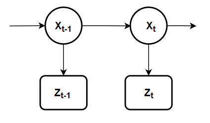
On the other hand, let me also say that the Kalman filter is one of the simplest dynamic Bayesian networks. It recursively calculates the true values of the states using incoming measurements and our mathematical model. Thus, our recursive Bayesian estimate also predicts the posterior distribution in the same way. In recursive Bayesian estimation, the true state is considered an unobservable Markov process. That is, measurements are considered observable states of our hidden Markov model, but this time, unlike the Hidden Markov Model, we work with continuous-time equations instead of discrete-time. As I said before, the true state at time $t$ is probabilistically conditioned only on the previous state ($t-1$) and is independent of earlier states. We express this mathematically as:

$$ p(x_t|x_{0},...,x_{N-1} ) = p(x_t|x_{t-1}) $$

and we can visualize the Markov chain as follows:

We can also visualize this recursive operation as information flow:

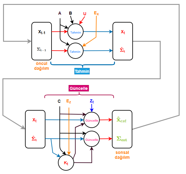
I will go into more detail about what happens from a Bayesian stochastic perspective and probability theory, but for now, let’s not confuse things and move on to coding what we’ve discussed above.

Coding the Algorithm

import numpy as np
import matplotlib.pyplot as plt
from math import *

# helper function to plot gaussian
def gaussianpdf(mean, variance, x):
    coefficient = 1.0 / sqrt(2.0 * pi * variance)
    exponent = exp(-0.5 * (x-mean) ** 2 / variance)
    return coefficient * exponent

# initialize meta variables
T = 15 # total driving time
dt = .1 # sampling period

# Let's assume we calculate the non-Bayesian position estimate using moving average
# The function below takes a signal and applies a moving average with a window of length 5
har_ort_length = 5
def smooth(x, window_len=har_ort_length):
    s = np.r_[x[window_len-1:0:-1], x, x[-2:-window_len-1:-1]]
    w = np.ones(window_len, 'd')
    y = np.convolve(w/w.sum(), s, mode='valid')
    return y

# define coefficient matrices (linear dynamic system coefficient matrices)
A = np.array([[1, dt], [0, 1]])  # state transition matrix - expected position and velocity of the car
B = np.array([dt**2/2, dt]).reshape(2,1) # input control matrix - expected effect of controlled acceleration
C = np.array([1, 0]).reshape(1, 2) # observation matrix - expected observations when state is known

# define main variables
u = 1.5 # magnitude of acceleration
OP_x = np.array([0,0]).reshape(2,1) # state vector representing position and velocity initialization
OP_x_est = OP_x # initial state estimate of the car
OP_acc_noise_magnitude = 0.05 # process noise - acceleration standard deviation - [m/s^2]
obs_noise_magnitude = 15 # measurement noise - autopilot sensor measurement errors - [m]
Ez = obs_noise_magnitude**2 # convert measurement error to covariance matrix
Ex = np.dot(OP_acc_noise_magnitude**2, np.array([[dt**4/4, dt**3/2], [dt**3/2, dt**2]])) # convert process noise to covariance matrix
P = Ex # initial estimate of car position variance (covariance matrix)

# initialize result variables
OP_position = [] # true position vector of the car
OP_velocity = [] # true velocity vector of the car
OP_position_obs = [] # observed position vector by autopilot

# run simulation from 0 to T with dt steps
for t in np.arange(0, T, dt):
    # calculate true state for each step
    OP_acc_noise = np.array([[OP_acc_noise_magnitude * i for i in np.array([(dt*2/2)*np.random.randn(), dt*np.random.randn()]).reshape(2,1)]]).reshape(2,1)
    OP_x = np.dot(A, OP_x) + np.dot(B, nu) + OP_acc_noise

    # create noisy observed position vector by autopilot
    obs_noise = obs_noise_magnitude * np.random.randn()
    OP_z = np.dot(C, OP_x) + obs_noise

    # store position, velocity, and observations as vectors for plotting
    OP_position.append(float(OP_x[0]))
    OP_velocity.append(float(OP_x[1]))
    OP_position_obs.append(float(OP_z[0]))

# plot true and observed positions of the car
plt.plot(np.arange(0, T, dt), OP_position, color='red', label='true position')
plt.plot(np.arange(0, T, dt), OP_position_obs, color='black', label='observed position')

# Classical statistical estimate using moving average instead of Kalman filter
plt.plot(np.arange(0, T, dt), smooth(np.array(OP_position_obs)[:-(har_ort_length-1)]), color='green', label='Classical statistical estimate')
plt.ylabel('Position [m]')
plt.xlabel('Time [s]')

plt.legend()
plt.show()

# Kalman Filter

# initialize estimation variables
OP_position_est = [] # autopilot position estimate
OP_velocity_est = [] # autopilot velocity estimate
OP_x = np.array([0,0]).reshape(2,1) # reinitialize autopilot state vector
P_est = P
P_magnitude_est = []
state_prediction = []
variance_prediction = []

for z in OP_position_obs:
    # prediction step
    # calculate new state prediction
    OP_x_est = np.dot(A, OP_x_est) + np.dot(B, nu)
    state_prediction.append(OP_x_est[0])

    # calculate new covariance prediction
    P = np.dot(np.dot(A, P), A.T) + Ex
    variance_prediction.append(P)

    # update step
    # calculate Kalman gain
    K = np.dot(np.dot(P, C.T), np.linalg.inv(Ez + np.dot(C, np.dot(P, C.T))))

    # update state estimate
    z_pred = z - np.dot(C, OP_x_est)
    OP_x_est = OP_x_est + np.dot(K, z_pred)

    # update covariance estimate
    I = np.eye(A.shape[1])
    P = np.dot(np.dot(I - np.dot(K, C), P), (I - np.dot(K, C)).T) + np.dot(np.dot(K, Ez), K.T)

    # store autopilot position, velocity, and covariance estimates as vectors
    OP_position_est.append(np.dot(C, OP_x_est)[0])
    OP_velocity_est.append(OP_x_est[1])
    P_magnitude_est.append(P[0])

plt.plot(np.arange(0, T, dt), OP_position, color='red', label='true position')
plt.plot(np.arange(0, T, dt), OP_position_obs, color='black', label='observed position')
plt.plot(np.arange(0, T, dt), OP_position_est, color='blue', label='Bayesian Kalman estimate')
plt.ylabel('Position [m]')
plt.xlabel('Time [s]')
plt.legend()
plt.show()

# define possible range of position
x_axis = np.arange(OP_x_est[0]-obs_noise_magnitude*1.5, OP_x_est[0]+obs_noise_magnitude*1.5, dt)

# Find Kalman state prediction distribution
mu1 = OP_x_est[0]
sigma1 = P[0][0]

print("Mean squared error: ", sigma1)

# calculate state prediction distribution
g1 = []
for x in x_axis:
    g1.append(gaussianpdf(mu1, sigma1, x))

# plot state prediction distribution
y = np.dot(g1, 1/np.max(g1))
plt.plot(x_axis, y, label='posterior prediction distribution')
print(np.mean(x_axis))
print(OP_position[-1])

# find observation distribution
mu2 = OP_position_obs[-1]
sigma2 = obs_noise_magnitude

# calculate observation distribution
g2 = []
for x in x_axis:
    g2.append(gaussianpdf(mu2, sigma2, x))

# plot observation distribution
y = np.dot(g2, 1/np.max(g2))
plt.plot(x_axis, y, label='observation distribution')

# plot true position
plt.axvline(OP_position[-1], 0.05, 0.95, color='red', label='true position')
plt.legend(loc='upper left')
plt.xlabel('Position [m]')
plt.ylabel('Probability Density Function')
plt.show()

If we run the above Kalman filter simulation, we get the following output:

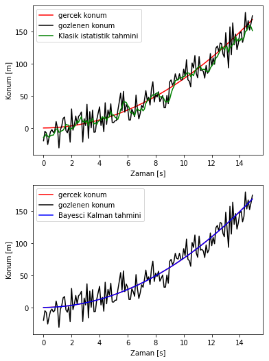
In the example, we not only used the Kalman filter but also considered a classical statistical method instead. Many classical statistical methods can be applied, but we used the moving average filter, which is frequently used in the literature for comparison.

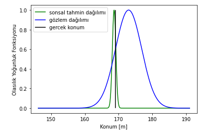
Finally, let’s look at the distribution of the last estimate made by the Kalman filter. As you can see, although the mean of the observation distribution (from GPS data) is far from the true position, the mean of the state prediction distribution is very close to the true position (with the simulation parameters above, our mean squared error is 0.274 meters!).

Advanced Topics and Real Life

Above, I mentioned the Kalman gain and gave the direct expression, but I did not say how it is derived. If you are curious about how the Kalman gain is derived, here is a hint: If you write the error covariance of the state prediction in matrix form and try to minimize the trace of this matrix, $Tr[\color{red}{\mathbf{\hat{\Sigma}_{t|t}}}]$, with respect to the Kalman gain, you can derive $\color{red}{K_t}$. Remember, the trace of the covariance matrix, i.e., the diagonal elements, gives us the mean squared error (mean squared error- MSE), and we are trying to minimize this error. If you want to see how the derivation is done, you can find it in this source from MIT: Kalman filter.

From another theoretical perspective, the main assumption of the Kalman filter is that the underlying system is a linear dynamic system, and the Kalman filter is theoretically optimal when the error and measurement random variables have Gaussian distributions (often multivariate Gaussian). The prior Gaussian distribution remains Gaussian after the linear transformations used in prediction. Therefore, the Kalman filter converges. But you may wonder: What if the dynamic system we are working with is not linear?

Then we need to use nonlinear functions instead of linear transformations. Nonlinear transformations can turn the prior Gaussian distribution into an unknown distribution. To get around such situations, “extended Kalman filters” have been developed. In the extended Kalman filter, the nonlinear function is linearized around the expected value of the current state estimate.

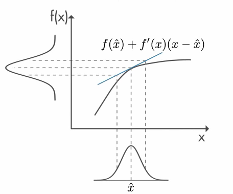
This figure is taken from Mathworks.

The nonlinear dynamic system is now modeled as follows:

$$ \hat{x}_{t} = f(\hat{x}_{t-1}, u_t) + \varepsilon_{x} \\ z_t = g(\hat{x}_{t}) + \varepsilon_{z} $$

To linearize this system, the following Jacobian matrices must be calculated.

$$ F = \left[ \frac{\partial f}{\partial x} \right ] _{\hat{x}_{t-1}, u_t}, G = \left[ \frac{\partial f}{\partial x} \right ] _{\hat{x}_{t-1}} $$

Now I have to say that, in real life, it is difficult to find and calculate the partial derivatives in these Jacobians analytically, and it is not always possible. Numerically calculating them is also computationally complex. On the other hand, the extended Kalman filter only works with models that can be differentiated, and if the system is highly nonlinear, it is no longer optimal.

When it is no longer reasonable or possible to solve with the Kalman filter, another famous algorithm comes to our aid, which slowly entered the engineering world from nuclear physics studies in the 1940s: Monte Carlo approximation. Since the 1990s, it has been successfully used to model nonlinear, nonparametric, and non-Gaussian dynamic systems. Monte Carlo filtering is also one of the most important algorithms discovered in this century! I will cover it in future posts.

Computational Complexity

The Markov property of Kalman filtering allows us to ignore the past beyond the previous state. Therefore, KF algorithms are advantageous in terms of memory and speed. This makes the Kalman filter a good candidate for embedded systems. Methods like Artificial Neural Networks, which are also candidates for solving the same problem, may require very long past data and are computationally much more complex. This means more memory and processing power. Therefore, they are not preferred in embedded systems.

References